INVESTING

Are Financial Planners Stuck in the 1970s?
By Martin Tarlie
Standard financial industry practice builds retirement portfolios using mean-variance optimization and validates them using Monte Carlo simulations that assume asset returns are a random walk. To put a finer, more brutal point on it, managers construct portfolios using technology from 1952 and then have the temerity to check the results using assumptions from 1970.
We suggest a more modern portfolio construction approach that puts the key problem of having sufficient assets to support investors’ required spending in retirement front and center.1 At the core of this approach is to define risk, not as volatility, but as “not having what you need when you need it.”
To effectively build a portfolio that minimizes the risk of “not having what you need when you need it,” we need models that understand how financial markets differ from the outdated academic assumptions of market efficiency and random walks.
Why Your Monte Carlo Is Wrong!
Conventional Monte Carlo simulation engines used by commercial financial planning tools assume that asset prices follow a random walk. But the empirical evidence based on real stock and bond returns over the past 100-plus years in the U.S. suggests random walk models overstate the long-horizon volatility of stocks and understate that of bonds.
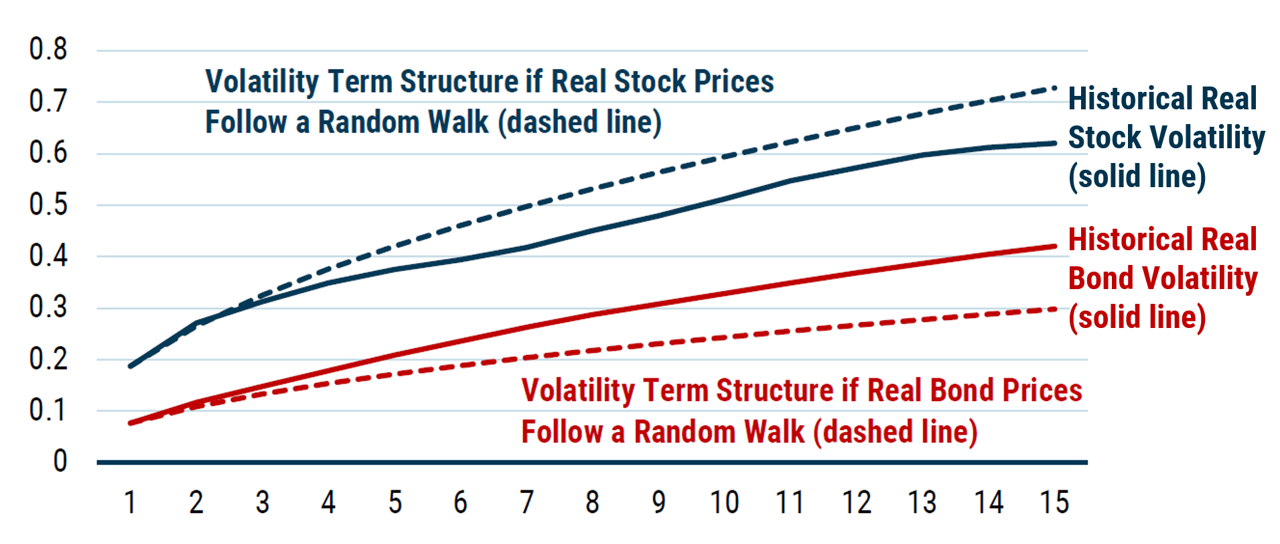
The empirical evidence is displayed in the following figure, which compares the empirical volatility profile of stocks and bonds (solid blue and red lines) with the volatility profile of a random walk model (dashed red and blue lines).2 Clearly evident is the fact that the random walk overstates long-horizon stock volatility and understates long-horizon bond volatility.
Exhibit 1. Volatility Profile of Stocks and Bonds: Historical versus Random Walk

While the empirical evidence is strong, the inherent volatility of returns means it is problematic to rely entirely on empirical evidence, even with 100 years of data. Consequently, we supplement the empirical evidence with models that explain the underlying mechanisms. For stocks, the mean reversion of valuation generates a volatility profile that rises more slowly than the random walk profile. For real bonds, the inverse relationship between unexpected inflation and real bond yields generates a volatility profile that rises more rapidly than the random walk profile. These models give us confidence that we are capturing real economic effects and not simply a statistical fluke.
Why Does This Matter?
Overstating long-run stock return volatility and understating long-run bond volatility has two effects. First, portfolios built based on the random walk paradigm tend to be bond heavy. In a world with time-varying expected returns, such bond-heavy portfolios have a negative impact on long-term outcomes.
Second, running Monte Carlo simulations with these flaws distorts viability and comparison tests. Such tests generate ranges of outcomes that are too wide for stock-heavy portfolios and too narrow for bond-heavy portfolios. It is precisely this type of analysis that can lead to bond-heavy portfolios in the first place.
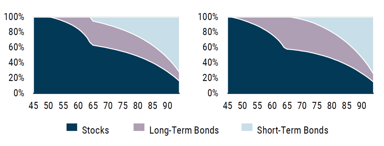
As an example of the first problem, the following figure compares two glide paths. The glide path on the left accounts for the empirical volatility profile we see for stocks and bonds, and the glide path on the right uses the counterfactual random walk model. Clearly evident in the right-hand glide path is the bond-heavy nature of the random walk approach—at age 65, the assumed retirement age, bond weight is about 60%. By comparison, the left-hand glide path has about 40% in bonds at age 65.
Exhibit 2. Portfolio Glide Paths: Historical Data versus Random Walk

What Can We Do about It?
Addressing the problem of Monte Carlo simulations that overstate stock volatility and underestimate bond volatility is fairly straightforward. One simply needs to model the return-generating process using time-varying expected returns that capture the underlying economic mechanisms.3
Fixing the problem of bond-heavy portfolios is more challenging. That’s because conventional portfolio construction methodologies are unable to account for such effects. The standard mean-variance paradigm that underpins Modern Portfolio Theory is a single-period framework and is therefore unable to incorporate the multiperiod characteristics that are necessary to address the underlying issue.
The problem with the conventional approach is that it is based on the notion that risk is volatility. But the real long-term risk you face is not volatility; it is “not having what you need when you need it.” The question needs to be reframed in terms of this real risk. This reframing leads naturally to an expected-shortfall approach to portfolio construction that, when married with a return generation process for real equity and bond returns consistent with historical market characteristics, solves the bond-heavy portfolio problem.4
To illustrate the effect this can have on long-term outcomes, we run Monte Carlo simulations that start with a 65-year-old who has just retired with $1 million in real terms. We then project 30 years into the future at various constant spending rates and ask whether the retiree runs out of money at any point over the 30-year period.
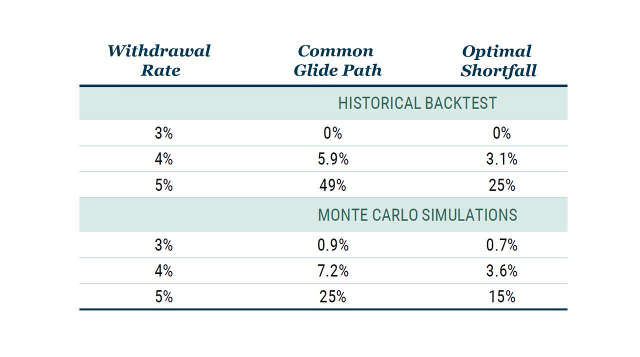
The following table compares the probability of ruin (i.e., running out of money) for two glide paths: (1) a “Common Glide Path” which is bond heavy and consistent with the random walk approach; and (2) an “Optimal Shortfall” that minimizes the risk of not having what you need when you need it but also accounts for mean reversion and empirically consistent volatility profiles. We see clearly that, both in historical backtests and Monte Carlo simulations, the optimal shortfall approach substantially reduces the probability of ruin for a variety of withdrawal rates.
Exhibit 3. The Risk of Running out of Money in Retirement:
Outcomes for Common Glide Path versus Optimal Shortfall Glidepath

Conclusion: A Better Way
The assumption of the return-generating process following a random walk for both stocks and bonds is ubiquitous in retirement planning, but it is rarely, if ever, examined or questioned. The rationale for using this assumption is stuck in the conventional wisdom of the 1970s, when the academic literature was generally characterized by belief in the random walk hypothesis. As Keynes long ago noted, “Practical men who believe themselves to be quite exempt from any intellectual influence are usually the slaves of some defunct economist.”
However, the academic world has moved on. Predictability is one of the “new facts in finance,” to borrow the phrasing of John Cochrane, a senior fellow of the Hoover Institution. The ideas presented here tie in with these views on predictability and suggest a way of modeling the return-generating process that is consistent with the empirical evidence, offers insights into the economic foundations and mechanisms that generate the returns, and, most importantly, provides a framework for portfolio construction that minimizes the risk of “not having what you need, when you need it.”
1. This article is based on the white paper “Investing for Retirement II: Modeling Your Assets.”
2. Data from 1926-2019 | Source: Online Data – Robert Shiller (yale.edu)
Solid lines are calculated using historical returns (i.e., volatility for a five-year horizon is the standard deviation of all five-year returns, including overlapping returns). Dashed lines are calculated by taking the one-year return volatility and multiplying it by the square root of the return horizon. Horizontal axis is the return horizon in years.
3. References for such an approach include the “Investing for Retirement II: Modeling Your Assets” whitepaper, and the more technical paper “Investment Horizon and Portfolio Selection.”
4. See https://www.nebo-gmo.com/insights#whitepapers for details on operationalizing a minimal shortfall approach to portfolio construction.
Dr. Tarlie is a member of GMO’s asset allocation team and Nebo product lead. Nebo is an innovative goals-based investment platformthat melds financial planning and asset management and implements the ideas in this article, among many others.
image credit: istock.com/selimaksan